Random Projections for Neural Networks
Random Projections for Neural Networks
Variance and the CLT
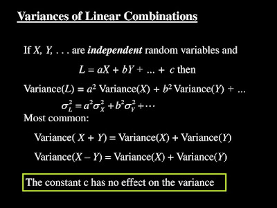
For Linear Combinations of Random Variables a negative sign before a particular variable has no effect on variance.
And of course the Central Limit Theorem is in operation.
The Walsh Hadamard transform (WHT) is a set of orthogonal weighted sums (where the weights are +1 or -1 or some constant multiple of those.)
And so the variance equation for linear combinations of random variables applies (minus signs not invalidating that), as does the Central Limit Theorem.
 |
| 8-Point Walsh Hadamard transform. |
If you want to use that behavior to generate Gaussians you should remember that the WHT leaves vector magnitued (length) unchanged (except by a constant c.)
The result is all the Gaussians are very slightly entangled through that property.
Destructuring the WHT
The reason the WHT can work as an image compression algorithm is that the underlying sequency (cf. frequency) patterns match strongly with patterns always found in natural images.
 |
| Sequency Patterns of the 8-point WHT. |
However that is a property easily broken by applying a random pattern of sign flips to the input data to a WHT or applying a random permuation.
What is left then is the residual variance and central limit theorem properties.
The combination of random sign flipping and the WHT then is a Random Projection (PR) of the input data. A transformation from the coherent domain into an incoherent domain of Gaussian noise.
If you know the original pattern of sign flips you can invert the Random Projection since both the WHT and sign flipping are self-inverse.
Neural Network Applications
You can use random projections for dimension reduction and dimensional increase.
Dimensional reduction and restoration via iterative smoothing is one option for processing large images with small neural networks.
Iterative smoothing shows there is a lot more information in random projection sub-sample than you might imagine and actually there is even more since by preforce smoothing loses high frequency information.
You can use random projections as form of preprocessing for neural networks. Especially for auto-associative neural networks.
Or you can use a random projection for fair splitting of input data between multiple small neural networks.
Binarizing the output of a random projection give you a Locality Sensitive Hash (LSH.) Where the output of the LSH is random but small changes in the input cause only a few bit changes in the output.


If we remember Rader's work on the FFT algorithm in 1968:
ReplyDeletehttps://en.wikipedia.org/wiki/Rader%27s_FFT_algorithm
He also did work on the Walsh Hadamard transform in 1969:
https://archive.org/details/DTIC_AD0695042
Where he used the WHT to generate random numbers with the Gaussian distribution.